Update 3: We Added GARCH Volatility Modelling to the Winning Strategies. A Quant's Adaptation.

So far this series has been about signals: which rule decides when to be long or short. This update is about the other half of trading that beginners ignore and professionals obsess over, which is how much to bet. We took the strategies that actually earned their keep across our tests and bolted a real quant tool onto them, GARCH volatility modelling, to see whether smarter position sizing makes a good strategy better. We did not change a single entry or exit. We only changed the size of the bet, and we let the data tell us whether it helped.

What we are actually doing

Every position has two parts: a direction and a size. Our earlier articles obsessed over direction. But your risk on any given day is roughly your position size multiplied by the market's volatility. If you hold the same size while volatility doubles, your risk just doubled without you deciding anything. That is the problem volatility targeting solves. Instead of betting a fixed size, you bet a size that is inversely proportional to how volatile you expect the market to be. When a storm is coming, you shrink the position. When the water is calm, you let it run. The goal is a roughly constant risk per day rather than a constant position.

To do that well you need a forecast of tomorrow's volatility. A naive approach uses a simple rolling standard deviation of recent returns, but that reacts slowly and weights a calm month and a violent one equally. GARCH does the job properly.

What GARCH is, in plain terms

GARCH stands for Generalised Autoregressive Conditional Heteroskedasticity, which is a mouthful that hides a simple observation: volatility clusters. Calm days tend to follow calm days, and violent days tend to follow violent days. Markets do not switch from sleepy to chaotic at random; turbulence arrives in stretches. GARCH is the standard model that captures this.

The workhorse version, GARCH(1,1), forecasts tomorrow's variance from just two things: how big yesterday's move was, and how volatile things already were.

sigma_t^2  =  omega  +  alpha * (yesterday's return)^2  +  beta * sigma_(t-1)^2

  omega  a small baseline level of variance
  alpha  how strongly a fresh shock bumps up volatility
  beta   how persistently past volatility carries forward

The alpha term makes the forecast jump the moment a large move lands. The beta term makes that elevated volatility fade slowly rather than vanish overnight, which is exactly how real markets behave. Together they mean-revert toward a long-run average, so after a shock GARCH predicts elevated but slowly-calming volatility, and after a quiet stretch it predicts continued calm. In Python, the `arch` library does the heavy lifting.

from arch import arch_model

# daily close-to-close returns, in percent (e.g. pct_change * 100)
model = arch_model(returns, mean="Zero", vol="GARCH", p=1, q=1)
res = model.fit(disp="off")

# one-day-ahead forecast of volatility (standard deviation)
fc = res.forecast(horizon=1, reindex=False)
next_day_vol = float(fc.variance.values[-1, 0]) ** 0.5

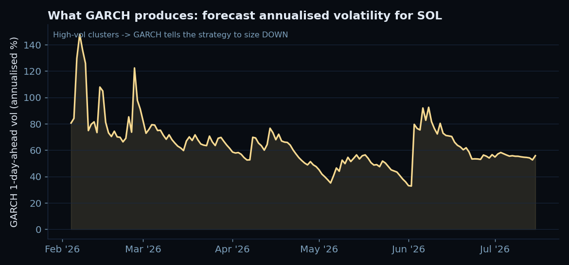
Here is what that forecast actually looks like on SOL over our window. Notice the clustering: volatility does not wander randomly, it ramps up and calms down in waves, which is precisely the structure position sizing can exploit.

How we sized the trades

We ran a rolling, out-of-sample forecast. On each day, GARCH was fit only on returns from before that day, so there is no lookahead. We turned the forecast into a position multiplier and left the entry signals untouched.

target_vol = returns.std()                        # a fixed daily risk budget
leverage   = (target_vol / next_day_vol).clip(0.3, 2.5)
position   = signal * leverage                    # signal is +1 / -1 / 0 from the strategy

We deliberately set the target so that average leverage stays near 1x. That is important: it means we are not secretly adding or removing risk overall, we are only moving risk from the volatile days to the calm ones. If GARCH sizing helps under those conditions, the help comes purely from better timing of exposure, not from cranking leverage. We applied this to three proven winners from the series, RSI(14) reversion (our most consistent strategy), EMA crossover (the big trend winner on SOL), and Bollinger breakout, across SOL, BTC, and NVDA over the same February to July window.

The results

Asset  Strategy              Return         Sharpe          Max drawdown
                           base -> GARCH   base -> GARCH     base -> GARCH
--------------------------------------------------------------------------
SOL    RSI(14) reversion    +23%  +25%     1.12  ->  1.29    -18%  ->  -17%
BTC    RSI(14) reversion     +7%  +10%     0.57  ->  0.82    -17%  ->  -16%
NVDA   RSI(14) reversion     +7%   +7%     0.62  ->  0.62    -20%  ->  -20%
SOL    EMA crossover        -35%  -32%    -1.20  -> -1.02    -47%  ->  -45%
BTC    EMA crossover        -21%  -25%    -0.88  -> -1.12    -37%  ->  -39%
NVDA   EMA crossover        -19%  -19%    -0.97  -> -0.97    -23%  ->  -23%
SOL    Bollinger breakout   -25%  -28%    -1.05  -> -1.06    -32%  ->  -41%
BTC    Bollinger breakout   +18%  +18%     1.24  ->  1.24    -12%  ->  -13%
NVDA   Bollinger breakout    -3%   -3%    -0.03  -> -0.03    -21%  ->  -21%

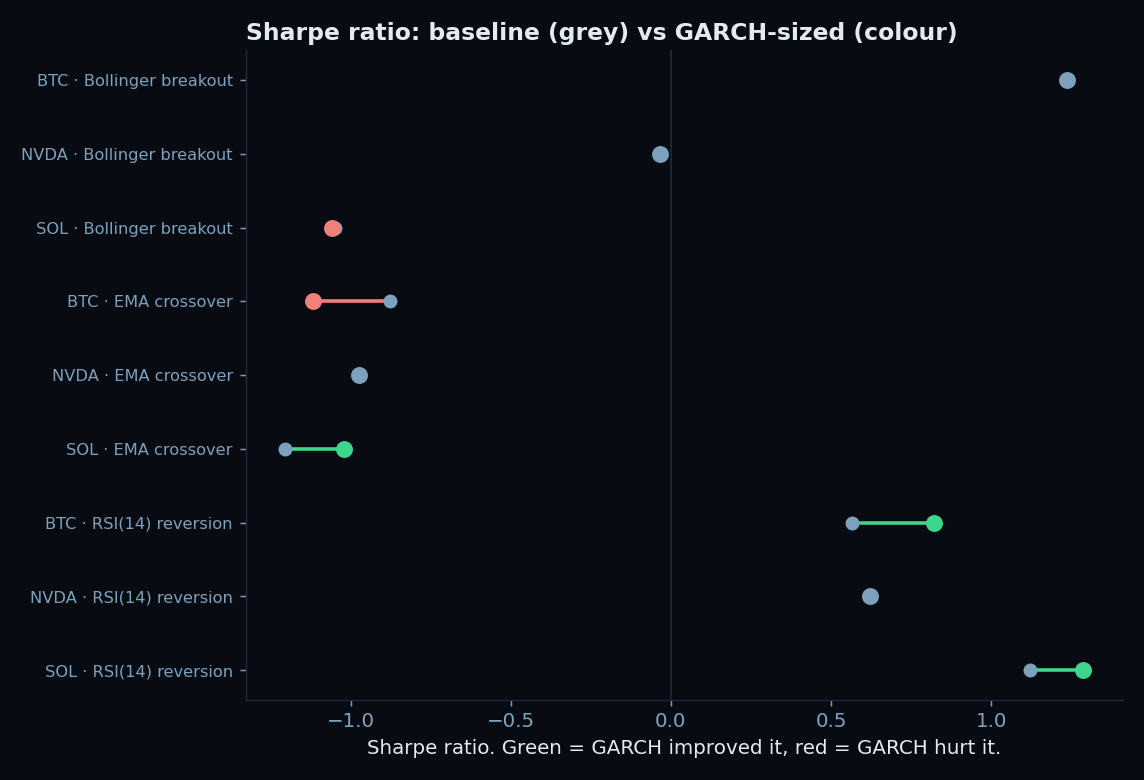
The honest headline is that GARCH is not a magic upgrade. Averaged across all nine cases it barely moved the needle, a Sharpe change of about +0.04 and, if anything, marginally deeper drawdowns on average. Anyone selling GARCH as a button that makes any strategy better is overselling it.

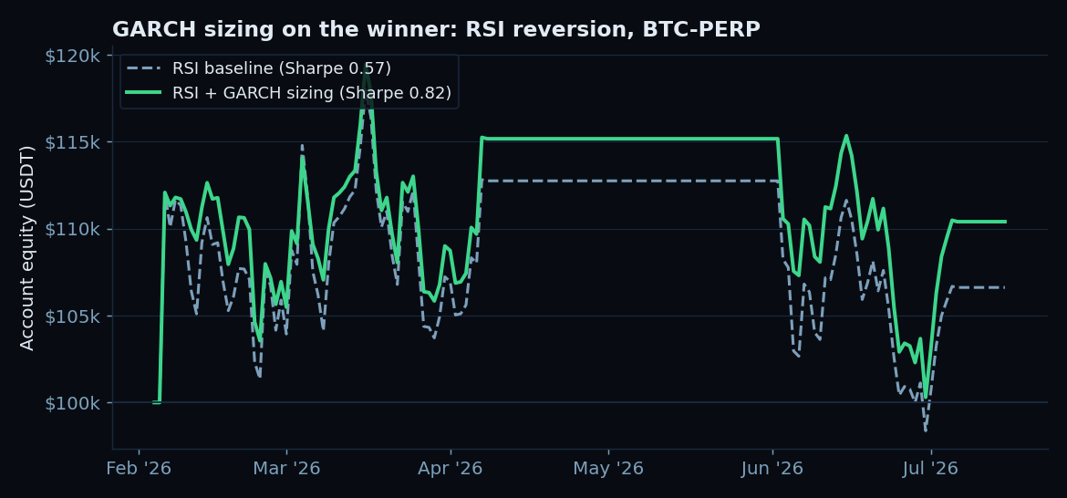
But look closer and there is a real, coherent pattern. GARCH sizing clearly and repeatedly helped the mean-reversion winner. RSI(14) reversion improved on both assets where volatility actually moved enough to matter: on SOL its Sharpe rose from 1.12 to 1.29 with a shallower drawdown, and on BTC from 0.57 to 0.82 while turning +7% into +10%. On NVDA it did nothing, because NVDA's volatility over this window was stable, so there was simply nothing for the vol timing to exploit. For the trend and breakout strategies, GARCH was mixed to slightly negative.

Why it helped one style and not the other

This is the interesting part, and it is not a coincidence. Mean reversion and volatility are natural enemies. A reversion strategy makes its money betting that a stretched price snaps back, and the thing that destroys it is a volatility spike where the stretch keeps stretching. Those spikes are exactly what GARCH sees coming, so cutting size right as volatility ramps protects reversion where it is most fragile. That is why RSI improved on every asset where volatility was live.

Trend following has the opposite relationship with volatility. Its best days are often its most volatile ones, the big committed moves it is built to ride. Shrinking the position precisely when volatility is high can clip the winners that make the whole strategy work. So the same GARCH layer that shielded mean reversion quietly taxed the trend strategies. And NVDA delivered the third lesson on its own: when volatility does not really change, volatility targeting has nothing to do, and the GARCH version is identical to the plain one.

The takeaway

GARCH is a genuinely useful quant tool, but it is not a universal upgrade you staple onto any strategy for free. It is a risk-management layer, and it pays off when it is matched to a strategy whose main enemy is volatility. For our most consistent strategy, mean-reversion RSI, GARCH sizing improved risk-adjusted returns on every asset where volatility was actually moving, which is a real and repeatable result. For trend strategies it was neutral at best. That fits the lesson this whole series keeps teaching: there are no free upgrades and no universal answers, only tools that fit some situations and not others. The professional's edge is not knowing GARCH exists. It is knowing which strategy to point it at.

Run it yourself

Everything above is reproducible, and we would rather you checked our work than took it on faith. If you have the LMEX MCP server connected to Claude, the easiest path is to let Claude pull the candles for you: ask it to fetch the daily OHLCV for a market from the LMEX connector, then hand the rows to the script below. Not connected yet? The LMEX MCP server takes a couple of minutes to set up, and the source lives on GitHub. The script runs the RSI mean-reversion signal, forecasts volatility with a rolling one-day-ahead GARCH(1,1) model, sizes each trade inversely to that forecast, and prints the baseline against the GARCH-sized version.

Install the libraries first with `pip install arch pandas numpy`. The script leaves funding out for simplicity, so treat the printed numbers as indicative rather than an exact match to the study above.

# GARCH volatility-targeted backtest, from the LMEX.AI strategy series.
# pip install arch pandas numpy
import numpy as np, pandas as pd, warnings
warnings.filterwarnings("ignore")
from arch import arch_model

# 1. Candles from the LMEX MCP server. In Claude, just ask:
#    "pull 400 daily candles for SOL-PERP from the LMEX connector"
#    and paste the returned rows into `raw`. Each row is
#    [timestamp, open, high, low, close, volume].
raw = [
    # [1784073600, 77.83, 78.15, 76.98, 78.08, 11420698],
    # ... paste LMEX candles here ...
]
df = pd.DataFrame(raw, columns=["ts", "open", "high", "low", "close", "vol"])
df = df.sort_values("ts").reset_index(drop=True)
df["ret"] = df["close"].pct_change()

# 2. The strategy signal: RSI(14) mean reversion, our most consistent strategy.
def rsi(c, n=14):
    d = c.diff()
    up = d.clip(lower=0).ewm(alpha=1/n, adjust=False).mean()
    dn = (-d.clip(upper=0)).ewm(alpha=1/n, adjust=False).mean()
    return 100 - 100 / (1 + up / dn)

def rsi_signal(df, n=14, lo=30, hi=70, mid=50):
    r = rsi(df["close"], n); pos = []; state = 0
    for v in r:
        if np.isnan(v): pos.append(0); continue
        if state == 0:  state = 1 if v < lo else (-1 if v > hi else 0)
        elif state == 1 and v > mid:  state = 0   # exit long
        elif state == -1 and v < mid: state = 0   # cover short
        pos.append(state)
    return pd.Series(pos, index=df.index)

# 3. Rolling one-day-ahead GARCH(1,1) volatility forecast. No lookahead:
#    each day is fit only on returns from before it.
def garch_vol(returns, minobs=60, win=150):
    r = returns * 100                     # scale up for the optimiser
    out = pd.Series(np.nan, index=returns.index)
    for t in range(minobs, len(returns)):
        window = r.iloc[max(1, t - win):t].dropna()
        if len(window) < minobs: continue
        try:
            fit = arch_model(window, mean="Zero", vol="GARCH", p=1, q=1).fit(disp="off")
            f = fit.forecast(horizon=1, reindex=False)
            out.iloc[t] = np.sqrt(f.variance.values[-1, 0]) / 100
        except Exception:
            pass
    return out

# 4. Backtest: fill next bar, charge 0.06% per side, compound.
COST = 0.0006
def backtest(df, position):
    pos = position.shift(1).fillna(0)
    turn = pos.diff().abs().fillna(pos.abs())
    net = pos * df["ret"].fillna(0) - turn * COST
    eq = (1 + net).cumprod()
    total = eq.iloc[-1] - 1
    sharpe = net.mean() / net.std() * np.sqrt(365) if net.std() > 0 else 0
    maxdd = (eq / eq.cummax() - 1).min()
    return total, sharpe, maxdd

# 5. Compare baseline sizing against GARCH volatility targeting.
signal = rsi_signal(df)
gvol = garch_vol(df["ret"])
target = np.nanmedian(gvol)                             # keeps average leverage near 1x
leverage = (target / gvol).clip(0.3, 2.5).fillna(1.0)   # size down when vol is high

for label, pos in [("baseline", signal), ("+ GARCH", signal * leverage)]:
    total, sharpe, maxdd = backtest(df, pos)
    print(f"{label:8s}: return {total*100:6.1f}%   Sharpe {sharpe:5.2f}   maxDD {maxdd*100:6.1f}%")

Ask Claude to pull BTC-PERP or NVDA-PERP candles instead to reproduce the cross-asset test, or drop in a different strategy signal in place of RSI to see whether GARCH sizing helps it too. If you want the funding-accurate, cost-exact version we ran, ask Claude to add the per-bar funding from the LMEX connector and to backtest on the common window, and it will extend the script for you.

Frequently Asked Questions

Q: Did GARCH make the strategies more profitable?

Not across the board. Averaged over all nine tests it was roughly neutral. But for the mean-reversion strategy, RSI reversion, it consistently helped, improving Sharpe and return on the two assets where volatility moved meaningfully and doing no harm on the third. For trend and breakout strategies it was mixed to slightly negative.

Q: Why does GARCH help mean reversion but not trend following?

Mean reversion is most vulnerable during volatility spikes, when a stretched price keeps stretching, so cutting size as GARCH forecasts a spike protects it. Trend following often makes its biggest gains on its most volatile days, so shrinking size then clips the winners it relies on. The same tool helps one and hurts the other.

Q: What is GARCH actually forecasting?

Tomorrow's volatility, specifically the conditional variance of returns. It assumes volatility clusters, so it blends how large the most recent move was with how volatile things already were, and mean-reverts toward a long-run average. It reacts faster and more sensibly than a plain rolling standard deviation.

Q: Did you use future data to fit the model?

No. The GARCH model was refit each day using only returns from before that day, and the forecast was for the next day. All position sizing was strictly out-of-sample, which is why the improvements, where they appear, are meaningful rather than curve-fitted.

Q: Should I add GARCH sizing to my bot?

If you trade a mean-reversion style, the evidence here says it is worth testing, since it improved risk-adjusted returns without changing your signals. If you trade trend following, test carefully, because vol targeting can trim the volatile winning moves you depend on. As always, validate on your own assets and timeframes before trusting it.

Related Articles